ABSTRACT //
For every fixed positive collar width, the separated regional pair in the scalar-field models considered here admits globally normal product states. We determine the sharp asymptotic order of the global mean-energy infima over PPT, separable, and product preparations as the collar width tends to zero. For the real scalar field in dimensions, , we proveThe Minkowski constants are uniform when remains bounded. The same law holds on bounded-geometry ultrastatic backgrounds with a uniform spectral gap. The lower bound applies to every globally normal state that is positive under partial transpose in the algebraic sense, including every separable state. A matching upper bound is furnished by globally normal quasifree Hadamard product states.
For the sharp regional momentum cross block, we also determine the least positive diagonal covariance required to erase it. Its curved-interface cost is uniformly for bounded , where is an explicit strictly decreasing mass-collar crossover function. At fixed mass the leading coefficient is independent of interface curvature and equals in .
The result is stable under approximation. Let be the uniform local witness gap produced by the proof. Exact membership in the PPT, separable, or product class, and every fixed-tolerance approximation with , have the same energy order. The lower proof combines a finite local PPT witness with an interface frame estimate controlled by the Hamiltonian. In dimensions, exact membership and every such fixed-accuracy approximation cost order . Microcausality remains exact; the law constrains preparation rather than transmission.
1 Introduction
Two spacelike separated regions carry commuting observable algebras. Their commutativity is the field-theoretic statement of causal independence. It is not statistical independence. A state is product only when every joint expectation factorizes, and it is separable only when it can be assembled as a convex mixture of such product expectations.
At positive separation, the split property permits normal product states. Buchholz established product states for suitably separated massive free-field algebras, and Sanders constructed separable quasifree Hadamard states on broad curved backgrounds [1–3]. At zero separation, tangent local algebras can be maximally Bell correlated and normal separable states can cease to exist [4, 5]. The unresolved boundary is quantitative. How much global energy is required to keep two regional algebras separable, or even close to the PPT set, when a collar of width is still positive but tends to zero?
Mode counting fixes the candidate ultraviolet scale. A collar resolves wavelengths of order , each carrying energy of order , while a smooth interface contains order independent cells. Their product is in three spatial dimensions. The theorem below turns this count into a regulator-free optimization law. Bény and coauthors anticipated the boundary-over-cutoff scale in a lattice productization argument, while Hollands and Sanders combined dilation with full-density interface packing to bound entanglement measures of a fixed vacuum state [5, 6]. Sanders’ planar translation-invariant competitors have finite energy density but infinite total energy; finite-total-energy separable Hadamard states for bounded regions were left open [3]. None of these results minimizes the global Hamiltonian over a state that may vary with the collar, or gives a regulator-free PPT lower bound matched by a finite-total-energy exact-product upper bound. A varying state can reorganize all of its correlations, so a fixed-vacuum estimate does not answer that optimization problem. To our knowledge, the construction and fixed-density frame estimate below provide the two matching bounds for the first time.
The main result proves the dimensional prediction without a regulator. It is also stronger than a separability bound. We minimize over the algebraic PPT class introduced by Verch and Werner [7]. This class contains every separable state. Its use avoids any tensor-product assumption for type III local algebras.
The proof has a lower half and an upper half, and the two halves use different ideas. The lower half begins with one finite local witness. Moving its expectation from the vacuum side of the PPT boundary to the PPT side forces a fixed occupation of the finitely many one-particle modes seen by that witness. Translations of those mode spaces along the interface form a Bessel family, whose total number operator is bounded by . This gives the local energy countA smooth interface supplies a full-density family of order cells. A state that is PPT on the full regional pair must neutralize the witness in every cell, which forces the cubic law.
The zero threshold in Eq. (1) is not essential. If a measurement protocol tolerates residual witness negativity , the same argument replaces the vacuum gap by . Averaging the cell witnesses then converts the count into an intrinsic state-norm distance from the full PPT set. Consequently, no fixed finite-energy state can be PPT, or remain within any fixed accuracy below the witness gap, at all sufficiently fine spatial resolutions.
The decisive phase-space fact is that the frame constant does not deteriorate as the number of interface cells grows. Dybalski’s sharpened nuclearity estimates controlled discrete sums of translated local excitations when increasing mutual separation suppressed their off-diagonal terms [8, 9]. Here the cell separation remains . By resolving only the finite modes seen by the PPT witness, the one-particle estimate remains uniform at the full interface density .
The upper half is constructive. An exact heat-kernel factorization of the two vacuum cross-covariance blocks produces a positive covariance correction whose off-diagonal entries cancel the vacuum cross terms. We prove separately that this correction is trace class in the vacuum one-particle topology, is the covariance of a Radon Gaussian distribution of coherent displacements, and has finite mean energy. Its Weyl characteristic functional factorizes on the two regional algebras, so the resulting globally normal Hadamard state is exactly product. Its energy is at most . A flat-interface calculation gives an explicit massive upper function. The exponent is therefore optimal.
On ultrastatic backgrounds, the Hadamard tangent limit and curved frame replace exact dilation and translation, while the heat-semigroup completion supplies the upper bound. For the separate constrained problem of positive diagonal erasure of the sharp momentum block, a boundary-Hankel calculation determines the exact flat crossover coefficient and its curved-interface asymptotic.
Sections 4–6 prove the lower bound and robust exclusion law. Section 7 constructs the matching product state. The appendices supply the operator-algebraic witness approximation, the curved frame estimates, the trace-class completion integral, and the boundary-Hankel calculus.
2 Regional states and the energy problem
Let be a local net in a vacuum representation on . Spacelike separation givesThe notation means the von Neumann algebra generated by the two commuting algebras.
A state is product across whenIt is separable when it belongs to the weak-star closure of the convex hull of product states. We use the weak-star closure because it is intrinsic to the algebras and includes the usual norm-closed normal separable class.
The algebraic PPT condition requiresfor every finite choice and [7]. It reduces to positivity of the partial transpose for matrix algebras. Every separable state obeys Eq. (4).
Let be the global Hamiltonian and let be a globally normal density state. Its mean energy isFor a regional pair depending on , defineThe infimum of an empty set is . The construction in Section 7 proves that the product set is nonempty at every positive collar in the models considered here.
Approximation requires a distance which remains meaningful for type III algebras. For a bounded linear functional on a von Neumann algebra , its norm isFor density operators in finite dimensions this is the trace norm of their difference, without the conventional factor . Operationally, any single observable with gives a lower bound on this distance. LetFor , let denote the corresponding set of states relative to that ordered pair of commuting algebras, and defineand, for ,The competing state need not possess a density operator or a global normal extension. This makes Eq. (11) stronger than a comparison restricted to normal regional states. Because , the distances obey . Each algebraic-PPT inequality is a weak-star closed linear inequality in the state. The PPT set is therefore convex and weak-star closed. The product set is closed by Eq. (3), and the separable set was defined with its weak-star closure. All three sets are consequently norm closed, so distance zero recovers exact membership.
We set until Section 9. In spatial dimensions, let be a complete Riemannian manifold. We write for -dimensional Hausdorff measure and set .
Regular collars.
A regular collar is specified by a compact nonempty smooth two-sided hypersurface with positive tubular radius. In Fermi coordinates , the two spatial regions have the formThe regions are relatively compact. Outside the tubular neighborhood , their closures remain at a fixed positive distance. Uniform perturbations with positive reach and bounded Jacobians obey the same estimates. This is a geometric condition; no witness-cell collection is supplied as a hypothesis.
Uniform families.
Family-uniform constants require common positive lower bounds on the injectivity and tubular radii, and uniform bounds on curvature, local interface graphs, Fermi Jacobians, and the derivatives of the potential used below. These bounds control both cell packing and overlap. For the upper construction, the fixed-distance parts of the cutoff supports must have volume at most and uniform cutoff seminorms. The same hypotheses give a common positive lower bound on every interface area. No upper area, intrinsic-diameter, or global annular-growth assumption is needed. For a single fixed interface the support conditions are automatic, and its fixed-distance terms are absorbed into the displayed law after reducing .
The spacetime regions are the causal developments of and . In Minkowski spacetime, is Euclidean and the scalar one-particle energy isHere denotes bosonic second quantization of a one-particle operator. On an ultrastatic spacetime , letWe assume bounded geometry of all orders, meaning a uniform positive injectivity radius and uniform bounds on curvature and its derivatives. We also assume a positive tubular radius and uniform bounds on all derivatives of . Closed is included. The spectral gap is used only to control the global infrared sector. The Minkowski theorem below also covers the massless case without a gap.
3 The sharp interface law
Theorem 1 Sharp interface energy lawLet and let form a regular collar along .
In the real scalar field on -dimensional Minkowski spacetime, fix . There are constants such that for every and every with ,
The same estimate holds on the ultrastatic scalar theory Eq. (15). Its constants are uniform on families with a common positive spectral gap, injectivity and tubular radii, uniform curvature, potential, local-interface, Fermi-Jacobian, and cutoff-seminorm bounds, and fixed-distance cutoff volume at most .
More precisely, the proof produces local selfadjoint contractions , with , and uniform constants . Every PPT state has , while the vacuum has . Every globally normal state of finite energy obeysThe interface family contains at least cells. Hence every fixed finite-energy state satisfies in every cell once is sufficiently small.
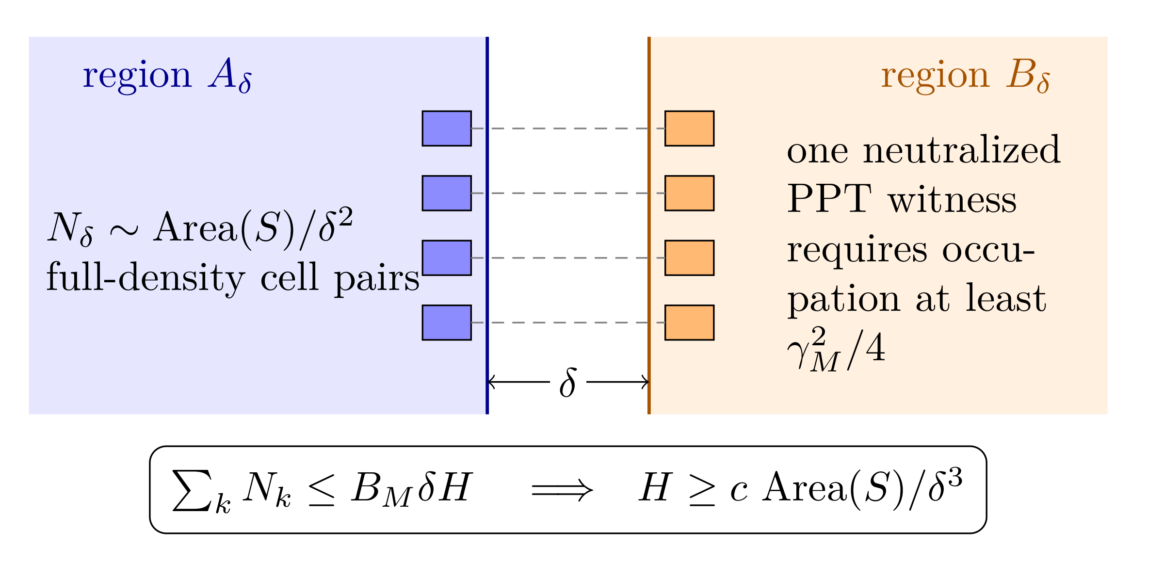
Corollary 2 Energy-constrained PPT exclusionUnder the hypotheses of Theorem 1, there are constants such that every globally normal finite-energy state obeysHere . The same conclusion holds with the corresponding uniform constants on the ultrastatic families covered by the theorem.
Consequently, if and , thenThe distance to the separable or product set is no smaller. The same energy bound therefore holds when the regional state lies within distance of either of those smaller classes. Since an exact product competitor has distance zero from all three classes, the complete robust law is
The power is sharp. In , the theorem readsThe lower constant is a finite-mode witness constant. It is independent of Gaussianity. The upper constant comes from an explicit product covariance. They need not agree.
Corollary 2 shows that exact equality is not driving the divergence. Any fixed approximation tolerance leaves the exponent unchanged. The dimensionless ratio controls how closely the regional state can approach the PPT set.
The square root in Eq. (18) has a concrete origin. A small vacuum–excitation superposition can change the expectation of a bounded witness by the square root of its occupation probability. A linear correction would therefore be false for unrestricted states. The proof keeps this dependence rather than hiding it inside an unspecified continuity constant.
The lower bound now reduces to two quantitative statements. Changing a bounded finite-mode witness by a fixed amount requires a fixed expected occupation of those modes. The translated occupations are bounded by . The next three sections prove these statements and count the interface cells. Section 7 then constructs the matching product state.
4 One finite witness and its occupation cost
4.1 Why the witness is chosen in a derivative subnet
An arbitrary compactly supported scalar smearing can carry a zero-momentum component. After multiplication by , translated copies of such a mode need not form a Bessel family on a two-dimensional interface. Without removing this zero-momentum obstruction, a uniform full-density frame bound fails. We remove it at the source.
Write a real Cauchy datum as , and denote the one-particle Hilbert space by . In Minkowski spacetime its one-particle vector isChoose an integer large enough that , and restrict the local Weyl generators to dataLet be the subnet generated by these derivative Weyl operators.
Proposition 3 Uniform finite derivative-mode witnessFix two nonempty, relatively compact, spacelike separated reference cells and a compact mass interval . There is a finite collection of selfadjoint derivative-Weyl polynomials such that, for each in that interval, one member satisfiesHere the displayed subscripts are to be read at the selected mass ; after normalization the gap may be chosen uniformly,The second constant is a common bound for the finite Gram inverses. The frame constant is derived from it in Section 5. On every bounded-geometry ultrastatic family in Theorem 1, the rescaled flat massless witness defines, in each sufficiently small Fermi cell, a finite Weyl polynomial which, after one family-uniform scalar normalization, is a selfadjoint contraction with the same PPT positivity and a uniform negative ground-state expectation.
The proof has four steps. First, the derivative subnet is still local and nonabelian. Second, its translated one-particle spaces are dense, so the usual analytic-continuation proof gives the Reeh–Schlieder property. Third, Theorem 6.2 of Verch and Werner then supplies completely positive maps from two qubit algebras into the two local algebras whose vacuum output is NPT [7, Thm. 6.2]. Finally, the maps can be approximated through their positive Choi matrices, not entry by entry. This last choice preserves complete positivity exactly while replacing all local operators by finite Weyl polynomials.
Appendix A checks these four points and the compact-mass uniformity. In the curved case, the same finite Choi sum-of-squares formulas remain completely positive for the local CCR. The Hadamard tangent limit is used only to transport the strict negative vacuum expectation [10]. Thus the algebraic PPT inequality and the vacuum-gap estimate enter by logically separate routes.
Negativity of is stronger than nonseparability. It certifies failure of algebraic PPT through fixed local operations. The construction uses no massive dilation symmetry; time-zero Weyl relations identify the algebraic polynomial across masses, while vacuum expectations and finite Gram matrices vary continuously with .
4.2 A finite-mode witness has a finite occupation price
Let be the finite-dimensional complex one-particle span of the Weyl arguments appearing in . Bosonic Fock space factorizes asThe witness acts only on the first factor. Let be the one-particle projection onto and letbe its number operator. Here denotes second quantization of a one-particle operator.
For an arbitrary globally normal state , denote the reduced density operator on by . Its vacuum vector is . The probability of leaving the finite-mode vacuum is bounded by the expected number,The trace-norm estimate against a pure state then givesThe subscript denotes the trace norm. Since and the vacuum expectation is at most , the same estimate gives the state-independent inequalityThis is the quantitative link between a measurable witness value and the occupation of its finite mode space. It holds whether or not the witness has crossed the PPT boundary. If while , the witness expectation changes by at least . Since ,Thus every state that neutralizes the witness pays the uniform lower priceThis step assumes neither Gaussianity nor a particle interpretation for the regional algebras. counts only the finite global Fock modes used by the witness.
5 The energy-frame estimate
The occupation cost becomes an interface law only if the translated mode spaces can be added without overcounting. This is the role of the frame estimate.
For mass , let denote the finite one-particle span of the Weyl arguments in the chosen witness, and put . Let , , be an orthonormal basis of this space. Spatial translations on the one-particle space are denoted by . DefineBefore orthonormalization, Eqs. (22) and (23) give the explicit formThe finite Gram matrix is uniformly invertible on a compact mass interval after redundant arguments are removed. Its inverse square root therefore changes Eq. (34) only by uniformly bounded finite linear combinations.
For , differentiate the products rather than either factor separately. Their worst low-momentum multiplier is . The choice gives a mass-independent locally integrable majorant for all derivatives used below. At large momentum the test functions are Schwartz. It follows thatRepeated integration by parts gives
Let be a relatively separated subset of . Ambient packing bounds the number of its points in the th unit shell by . Hence Eq. (36) is summable in every row of the block Gram matrix indexed by . Schur’s test gives a constant independent of the number of points such thatSince , this is equivalent, as a quadratic-form inequality, toSecond quantization preserves positive form inequalities, so
Equation (38) is the new phase-space input. It controls only the finite modes which cross the PPT boundary. It does not attempt to cover the unit ball of a local algebra, and its coefficient is therefore independent of the number of cells.
6 From a regular interface to the lower law
6.1 The interface supplies the cells
Fix a small reference pair of positively separated spatial cells in . A regular collar supplies scaled copies of this pair without an additional packing assumption. Cover the compact interface by finitely many graph patches on which the unit normals lie in a fixed narrow cone. Choose one oriented reference pair for each patch and shrink it once so that literal translates fit on the two sides throughout that patch. Partition the interface among the patches, then choose one globally maximal set of points separated by in the induced metric. Assign each selected center to its designated graph patch and orientation. Take larger than the tangential diameter of every reference pair. Positive reach and uniform graph bounds place one translated pair at every chosen point and give uniformly bounded overlap across patch boundaries and distinct folds. Standard volume comparison on the compact hypersurface givesWithin each graph patch, the centers form a relatively separated Ahlfors family and the mode spaces are literal translates of one fixed oriented space. Equation (38) therefore applies patch by patch. Summing the finitely many frame bounds only changes the constant. This is exactly the geometric input used in the shell count below Eq. (36).
The assertion remains true for uniform collars. At scale , the graph error from the tangent plane is , while the free space inside a reference cell is . Reducing the fixed cell size once makes every copy fit for all sufficiently small collars.
6.2 Exact scaling in Minkowski spacetime
Let be the unitary dilation on the one-particle momentum space,and let . It maps the mass- reference theory to scale in the mass- theory. Direct substitution givesThis is an isomorphism between different mass theories. It is not a massive dilation symmetry.
Choose , with a fixed small enough that the scaled reference cells fit inside Eq. (13). The reference mass isThe condition keeps in a compact interval. After conjugating Eq. (38) by , the physical cell projections obeyDefine the corresponding physical cell number operators bySecond quantization yields
If the regional restriction of is PPT, its restriction to every cell pair is PPT. It therefore neutralizes every local witness. Applying Eq. (32) in all cells givesEquations (40) and (47) proveThis is the first inequality in Eq. (16).
For an arbitrary finite-energy state, fix a tolerance . Equation (30) shows that every cell satisfying must obeyApply Eq. (46) only to those cells. This gives the tolerant countAt , Eq. (50) is the exact neutralized-cell law claimed in Eq. (17). When its right side is smaller than one, every witness in the family remains below . The conclusion therefore survives a fixed measurement margin.
This count also controls approximation to PPT in each cell. Let be the state-norm distance between the restriction of to the th cell pair and that cell’s algebraic-PPT set. Since every cellwise PPT state has nonnegative expectation on ,ThereforeThe tolerant witness count is thus also a bound on how many interface cells can lie within distance of PPT.
6.3 Robust distance from the PPT set
The tolerant cell count has an intrinsic regional form. Average the witnesses over the interface,Each witness has norm at most one, so . If is any algebraic-PPT state on , its restriction to each cell is PPT. ThereforeThis remains true even when is singular or has no globally normal extension.
Write . Averaging Eq. (30) and applying Cauchy–Schwarz givesThe frame estimate and the geometric cell count now enter separately. Equations (46) and (40) yield
Equation (56) becomes a distance statement by observable–state duality. For every PPT state ,Taking the infimum over proves Corollary 2 withSolving Eq. (18) for gives Eq. (19). The exact lower bound is the special case . The derivation also explains the experiment represented by : choose one interface cell uniformly at random and perform its finite witness protocol. No collective type III measurement is required.
6.4 The curved one-particle frame
The flat proof used exact dilation to set the cell size and exact translation to compare different cells. Neither operation is a symmetry on a general ultrastatic slice. Fermi rescaling replaces the dilation, while a direct Sobolev synthesis estimate replaces translation invariance.
Work in Fermi coordinates centered at an interface point. Put on the fixed reference cell and define by . Let be the undifferentiated flat primitives used in Eq. (23). To keep the cell notation readable, denote their density-corrected rescalings by :The powers have separate roles. After is applied once, the -amplitude is and the -amplitude is . Thus the one-particle Gram matrix is scale invariant, whereas the energy-divided modes below have squared norm of order . The factor removes the leading volume distortion.
The corresponding one-particle vectors areLet be their span, choose an orthonormal basis , and put
Proposition 4 Uniform curved frameUnder the bounded-geometry, potential, gap, collar, and chart bounds in Theorem 1, there are , independent of the interface point and of the member of the controlled family, such that for :
the Gram matrices of the vectors have all eigenvalues in a fixed interval ;
on the form domain of ,
Appendix B proves both statements. The key estimate is local. For every finite coefficient array , the superposition of rescaled profiles has norm squared at most . The analogous superposition obeys the same bound in . Uniform ellipticity converts these estimates into a Bessel bound for the divided one-particle modes. Within-cell Gram conditioning then gives Eq. (63). The proof uses only bounded overlap of the witness supports and introduces no global shell or diameter assumption.
The same finite Choi sum-of-squares formulas built from the curved Weyl generators define CP maps in every cell. They preserve the algebraic PPT inequality exactly. The Hadamard tangent limit is needed only to transport the strict negative vacuum gap into every cell. Combining Eq. (63), the occupation cost, and Eq. (40) provesAll constants are uniform on the bounded geometric families stated in the theorem. The tolerant count and averaged-witness proof use only this frame inequality, the uniform gap, and the same geometric cell count. They therefore give Eq. (18) on the curved family with . No curved-space density matrix or regional tensor factor is introduced.
7 Matching product states
Sharpness requires exact product states at the same order. We now construct them.
7.1 Positive completion of the cross covariance
For the ultrastatic scalar vacuum, the symmetric equal-time covariance on real observable test data isChoose smooth cutoffs equal to one on and . Their supports remain at distance at least , and their th derivatives are . The cross covariance is the two-component smoothing operatorBoth entries in Eq. (66) mean the unique extensions of the off-diagonal distribution kernels, initially evaluated on compactly supported smooth data. They are not unrestricted compositions with the generally unbounded operator . The separated cutoff supports make both extensions smoothing.
The completion is easiest to see for one rank-one cross term. Let and be smooth classical mean configurations supported on the two sides. We writeIf a covariance contains the cross term and its transpose, then adding the positive squarecancels those cross terms and adds only positive diagonal covariance. The mean energy carried by that square is , whereThe heat-kernel construction below is an integral of this elementary operation.
Define the energy nuclear cost of the cross kernel bywhere the infimum is over smooth support-preserving expansionsHere and are supported on the and sides, respectively, and the energy sum in Eq. (70) is finite. The equality is an equality of bilinear forms on smooth regional test data, continuous in the energy projective tensor norm. The notation also includes Bochner integrals of rank-one forms; signs and finite component indices are absorbed into .
Extend by zero to global mean configurations and put . Every such expansion has the positive completionAdding to the vacuum covariance preserves the CCR uncertainty inequality. Its off-diagonal block is , so the new covariance has zero cross block on . At this stage this is a positive quasifree covariance form. Global normality, exact factorization of the regional state, and identification of its added mean energy with the selected completion cost are separate operator statements. They are proved after the heat estimate and in Appendix C. For the selected expansion, writeThe infimum of this quantity over all admissible expansions is .
The relevant estimate isIt follows from an exact heat-kernel factorization. Let be the kernel of and putThe semigroup identity givesSince , functional calculus gives the exact off-diagonal representationsThe two heat vectors in a rank-one term can have very different norms: one is controlled by the distance to and the other by the distance to . Multiplying one vector by a positive number and the other by its reciprocal does not change their tensor product. We use this freedom to balance the two diagonal costs. PutSaloff-Coste’s Gaussian estimate includes uniformly bounded lower-order terms, and the bounded-geometry derivative estimates cover the Laplacian [11, Thms. 6.1 and 6.5] [12, Thm. 4.1]. Uniform scaled interior parabolic estimates in normal charts extend the derivative bounds to the real potential under the coefficient bounds stated above. The argument in Appendix C also shows that one Gaussian exponent works for every spatial derivative order, while the prefactor depends on that order. For , defineFor , set . Reciprocal rescaling leaves every cross term unchanged, while the two Gaussian bounds acquire the same exponent, proportional toAdd the positive square built from in the field sector and from in the momentum sector. Their cross terms cancel Eqs. (77) and (78) exactly.
Gaussian heat-kernel and gradient estimates then givefor . The remainders come from the fixed-distance part of the regions and have -independent weighted integrals. The term is the cost of the cutoff gradients. For the Minkowski operator , the last factor in Eq. (83) is . The hypothesis absorbs the mass term into the same bound. The large- integrals converge by the spectral gap on the curved background. In massless Minkowski space they converge by the explicit Euclidean heat kernel and relative compactness of the regions. Consequently,It follows that also obeys Eq. (74). The two singular integrals areThe second estimate is the point at which enters the upper proof. Appendix C proves the overlap estimates. The part of the regions outside the tubular collar stays at fixed distance and contributes only .
For every fixed , differentiation in either kernel variable adds only powers of and . The scalar is independent of those kernel variables. The common Gaussian exponent in Eq. (80) therefore survives every derivative. All differentiated small- integrals converge, so the completed Cauchy covariance has a smooth compactly supported kernel. Its spacetime evolution is a smooth bisolution, whose wavefront set is empty. Adding it therefore leaves the Hadamard wavefront set unchanged [13].
Proposition 5 Normal coherent realization of the completionFor every fixed , the positive heat-kernel completion is the covariance of a centered Radon Gaussian distribution of coherent displacements in the vacuum Fock representation. Its coherent-state mixture is a globally normal density state with covariance . The state is Hadamard, is exactly product across and , and satisfiesThe constants have the uniformity asserted in Theorem 1.
Proof A real Cauchy datum has the ultrastatic one-particle representativeIn Minkowski spacetime, spatial Fourier transformation turns this into Eq. (22). A classical mean configuration determines the real one-particle displacementWith the Weyl convention of Eq. (22), conjugation by the Fock displacement multiplies by , with as in Eq. (67). The real one-particle norm and the coherent mean energy are
Regard the one-particle Hilbert space as a real Hilbert space with inner product . For the selected rank-one completion in Eq. (72), definewith the sum replaced by the corresponding positive integral for the heat decomposition. This is the precise real one-particle covariance induced by . It is trace class. In the gapped theory, Eq. (89) is bounded by . For Minkowski space, uniformly for every , all completion vectors have support in one fixed compact set and . The Riesz-kernel representation and the Hardy–Littlewood–Sobolev inequality giveby Hölder’s inequality [14]. This controls the momentum-displacement contribution to the one-particle norm. For a field displacement, Cauchy–Schwarz and the ordinary compact-support Poincaré inequality give, uniformly in , . Integrating these bounds against the positive rank-one decomposition and using Eq. (84) gives .
A positive trace-class covariance on a real Hilbert space determines a centered Radon Gaussian measure [15]. Let denote the real one-particle random variable with this law. The finite form trace also implies almost surely. Averaging the corresponding coherent vacuum vectors gives the Bochner integral in the trace classIt is positive, has trace one, and is globally normal by construction. Its Weyl characteristic functional isHerewhich follows from Eqs. (67), (88), and (91). This proves directly that the mixture is the centered quasifree state with the completed covariance. No separate quasi-equivalence argument is needed for normality because Eq. (93) is already a trace-class density operator in the vacuum representation.
For test data supported in the two regions, the completed cross covariance vanishes. Locality also gives . ThereforeFinite linear combinations of regional Weyl generators are norm dense in the regional Weyl -algebras. Kaplansky density and the normality of extend Eq. (96) separately in each variable to the two regional von Neumann algebras. Thus the regional state is exactly product in the sense of Eq. (3).
Finally, Tonelli’s theorem and Eq. (90) giveThe smooth-kernel argument preceding the proposition proves the Hadamard claim. This completes the proof. ◻
Proposition 5 proves the upper half of the main theorem and the nonemptiness of the product class at every positive collar.
Completion of the proof of Theorem 1 In Minkowski spacetime, Proposition 3, the flat frame inequality (44), and the geometric cell count (40) give the PPT lower bound in Eq. (48). Proposition 4 and the curved tangent witness give the corresponding ultrastatic lower bound (64). Proposition 5 supplies a globally normal exact-product competitor with the matching upper order in both settings. The inclusions give the two middle inequalities. The compact-mass construction in Proposition 3 and the uniform constants in the two analytic propositions give precisely the mass and bounded-geometry uniformity stated in the theorem. The count law is Eq. (50) at . ◻
8 Coefficient laws for covariance completion
8.1 Exact planar product completion
For an infinite planar interface, a translation-invariant completion yields an exact energy density. It is not the finite-total-energy competitor used in Theorem 1, but it exposes the coefficient as a function of . Take parallel half-spaces and and Fourier transform in the tangential directions. In , putThe two vacuum cross kernels have the following Laplace decompositions. Here and are modified Bessel functions of the second kind.whereEach rank-one term is completed by equal positive diagonal blocks. The field profile takes opposite boundary values on the two sides. Extending it by zero would create a jump and infinite gradient energy. Instead, continue it through the collar by the minimum-energy solution of . Its collar energy, before the Hamiltonian factor , isThe momentum profile has only an energy and needs no derivative matching.
Adding the field, collar, and momentum contributions gives the exact energy of this chosen fiber competitor,Define the tangential energy density by Fourier decomposition, equivalently as the energy per area in a large tangential torus followed by the thermodynamic limit. Integration over tangential momentum yieldsThe integral is finite. At , its coefficient isEquation (104) is the energy density of this translation-invariant half-space completion. Its total energy is infinite because the interface is infinite. The heat-kernel construction above supplies the globally normal finite-interface product states used in the theorem. The flat calculation independently displays the same cubic scale and gives an explicit massive coefficient.
8.2 Sharp momentum-block erasure and its curved limit
A related constrained minimization can be solved exactly: the least positive diagonal covariance required to erase the sharp momentum cross block. Its coefficient is distinct from the smooth product completion above and from the unrestricted separability optimum.
Take parallel half-spaces and let be the sharp spatial projections onto and . For mass , define the energy-weighted momentum cross operatorBecause need not preserve , Eq. (106) denotes the restriction of the off-diagonal distribution kernel, not a literal composition of unbounded operators. It is defined first on . Tangential Fourier transform gives a decomposable operator whose normal fibers are trace class; the full planar trace norm is infinite only because the interface area is infinite. Let reflect the half-line onto the half-line. After tangential Fourier transform, the fiber of is negative. Its negative is the positive Hankel operator with and kernelThe factor in Eq. (106) is included in this kernel. Positivity follows because the right side is a positive integral of the rank-one kernels . Hence its trace norm equals its trace,The ordinary trace norm is infinite because the interface is infinite. Define its tangential trace density byRescaling and gives the exact scaling formInterchanging the two positive integrals and evaluating the tangential ball gives the one-dimensional formulaThus Eq. (110) is exact throughout the scaling regime . The function is continuous and strictly decreasing on : increasing both shrinks the integration interval and strictly decreases on the surviving interval. At , the gamma duplication formula givesConsequently, for fixed , or more generally whenever ,In , the leading coefficient is
The trace norm has an exact positive-completion meaning. For a Hilbert space , write for the cone of positive trace-class operators on . If is trace class, thenIndeed, positivity gives with , so . Equality follows from the polar decomposition by choosing and . Applied fiberwise, this proves that Eq. (113) is the least positive diagonal noise needed to erase this one sharp momentum cross block.
The flat coefficient is the local model for a curved sharp interface.
Theorem 6 Sharp mass-collar crossover for momentum completionLet and the collar geometry satisfy the ultrastatic hypotheses of Theorem 1. For this result, assume in addition that the collar is . Fix an integer . In every admissible Fermi chart, impose uniform derivative bounds through order on the Fermi metric, its inverse, and the Fermi Jacobian, and through order on the second fundamental form. The fixed-distance pieces of the sharp regions have volume at most and uniform local geometry. A fixed smooth interface satisfies these conditions automatically. PutFixed curvature coupling is included by absorbing it into the smooth potential . There is , smaller than one quarter of the tubular radius, with the following property. For , define the sharp cross operator first on byPositive separation gives a unique trace-class extension . It is denoted schematically by , without asserting that the sharp projection preserves . Writing , its least positive diagonal completion cost isFor every , there are and such that, whenever and ,Consequently, if , thenFor fixed mass, or whenever , the leading coefficient is the universal value in Eq. (112). In it is . It is independent of the interface curvature, fixed curvature coupling, and smooth fixed potential.
Proof Equation (115) gives the exact completion identity. The trace-class boundary-symbol estimate in Appendix D compares the curved collar operator, in trace norm, with the positive flat normal Hankel model at every point of . Its phase-space trace is , and its remainder is the right side of Eq. (119). ◻
Theorem 6 exactly solves positive diagonal momentum-covariance erasure. The unrestricted separability problem is broader because a competing state’s covariance difference from the vacuum need not be positive; its sharp coefficient remains a separate interface-tension problem.
9 What the law means
9.1 Separability is an ultraviolet preparation condition
At every fixed , exact product states exist with finite energy. The divergence concerns the limit , not existence at a fixed positive collar. The number of independent interface cells grows like area divided by . Neutralizing the witness in one cell forces an energy charge of at least . The heat completion supplies the matching global upper law. The cell count and the per-cell charge are independent parts of the lower proof, and their product gives the sharp power.
For , restoring constants gives the scaleThe constants hidden in depend on the selected witness and on uniform geometric bounds. The power does not.
The robust form shows that this law is not created by demanding exact factorization. For every fixed , a state that comes within state-norm distance of the PPT or separable set pays the same power. Conversely, any family satisfyingremains a fixed positive state-norm distance from every PPT and separable state as the collar closes. The statement concerns the physical regional algebras. It does not declare abstract tensor products or finite-dimensional product density matrices inconsistent.
9.2 The local statement is stronger than the global divergence
The tolerant count law Eq. (50) is the operational core. For a fixed finite-energy state, its right side tends to zero. The state therefore violates the same pulled-back PPT witness by more than any fixed margin in every sufficiently small cell of the chosen full-density interface family. Each violation uses only finitely many Weyl observables in two spacelike separated cells. The local CP maps in the construction convert the violation into a two-qubit NPT output, so the certified correlation is one-copy distillable.
Dividing the count law by the number of available cells gives an operational fraction bound, measurable once the local witness has been calibrated:Here . In three spatial dimensions, the right side is proportional to divided by the interface area. A preparation of fixed energy can therefore bring only a vanishing fraction of the witness array within the chosen PPT tolerance. Every cell outside that fraction has and is certified NPT by the same finite measurement protocol.
The conclusion is not obtained from a nonzero two-point function alone. A separable mixed state may have connected correlations. The witness crosses the convex PPT boundary, which is why it proves nonseparability.
9.3 A nonflat example
Consider the Einstein static spacetimeThe curvature term gives a spectral gap even at . Let be a latitude two-sphere at polar angle . Its area isThe theorem gives, uniformly for ,This example shows that the mechanism is local to the interface and does not depend on global translation or dilation symmetry.
9.4 Finite free multiplets
The scalar law adds component by component.
Corollary 7 Finite free multiplet lawLet and consider independent real scalar fields with masses and total HamiltonianUnder the geometric hypotheses of Theorem 1, with and , if for every component, thenA constant positive semidefinite internal mass matrix is included by taking to be its eigenvalues. The same conclusion holds for a finite direct sum of the ultrastatic scalar operators in Eq. (15) when all components belong to one common uniform family.
Proof If the aggregate regional state is PPT, its restriction to the th field remains normal and PPT. The scalar lower bound applies to every component, and summing gives the left inequality without assuming independence between species. For the upper bound, take one scalar product competitor per component and regroup their tensor product by spatial region. Energies add. A constant internal mass matrix is diagonalized by a pointwise orthogonal field transformation, which preserves localization and the total Hamiltonian. The ultrastatic direct-sum statement is identical. ◻
9.5 Finite regulators and the continuum limit
Absolute separability remains a genuine spectral property in finite dimensions [16, 17]. There is no contradiction. A regulator contains only finitely many interface modes. As the cutoff is removed, the theorem says that keeping all of their regional PPT constraints forces the Hamiltonian expectation to follow the ultraviolet cell count. A sequence of regulated separable states can approach a normal continuum state only if it fails the regional PPT condition on an increasing set of ultraviolet cells, or if its energy diverges at the stated rate.
For a finite-mode bosonic regulator, the three energy problems have exact covariance formulations. Finite-mode means finitely many genuine canonical oscillator modes. Their Fock space is still infinite-dimensional. This is not a truncation to finitely many number states, which would destroy the exact canonical commutation relations.
Appendix E gives an exact covariance reduction for these regulated problems. For every finite collection of canonical bosonic modes and every positive quadratic Hamiltonian, the unrestricted PPT, separable, and product energy minima are semidefinite programs. Gaussianity is a conclusion of the reduction, not an assumption on the optimizing state. The continuum frame theorem fixes the scale these programs must obey under geometric refinement, but it does not prove convergence of their normalized optimal values. That separate limit is the interface-tension problem.
10 Relation to observable field correlations
Electro-optic sampling has measured vacuum-field cross correlations between spacetime sampling volumes, including contributions dominated by spacelike separation [18]. A later experiment resolved different optical quadratures and separated vacuum fluctuations from source radiation [19]. These measurements demonstrate that correlation and causal response can be resolved independently. They motivate an analogous scalar-mode test, but they do not establish nonseparability or test the scalar theorem.
The distinction is visible in the simplest two-mode inequality. For output modes , write and defineEvery separable two-mode state with finite second moments obeys[20, 21]. Cross-correlation and response traces do not determine the two local occupations on the right. The published electro-optic data therefore motivate the regional observable problem but do not already test Eq. (130) or the field witness .
The theorem fixes the experimental architecture; the remaining task is a finite calibration for the chosen apparatus. The existence proof passes through Reeh–Schlieder, one-copy distillability, and a finite approximation argument. Once explicit derivative-weighted mode profiles, Weyl-polynomial coefficients, and a certified witness gap have been computed, one can measure the Weyl moments entering each local witness and average the results over uniformly sampled interface cells. This samples without requiring one collective field measurement. If an experiment obtains an estimate with additive uncertainty andthen every PPT state is separated from the measured state by at leastThe witness therefore certifies a quantitative distance from PPT without full state tomography.
An independently calibrated upper bound on the global mean energy gives a second check. Equation (18) guarantees a negative witness margin wheneverRepeating the same mode geometry while reducing would then test the predicted interface scaling. Producing the explicit witness and calibrated constants is the missing practical step. It is a finite witness-construction problem rather than full field tomography. The proposed test concerns correlation and preparation energy; it requires no signal to propagate between the regions.
11 Conclusion and scope
The proof uses four ingredients. The first three are a uniform finite local PPT gap, a positive local excitation counter which pays for neutralizing that gap, and an interface frame inequalityThe fourth is a regular interface which supplies at least cells. Any continuum theory with analogues of all four ingredients obeys the same lower law, tolerant cell count, and state-norm exclusion from PPT. In the scalar field, the counter is a finite-mode number operator and Eq. (134) follows from the one-particle Bessel estimate. This is the structural part of the result and the precise target for extensions beyond quasifree fields.
For positive diagonal erasure of the sharp momentum cross block, the boundary-Hankel theorem goes further: it gives the exact crossover function and a curvature-independent fixed-mass leading coefficient. That coefficient belongs to the constrained covariance-completion problem; the unrestricted separability coefficient is the remaining interface-tension problem.
The law concerns global preparation energy in globally normal states of the stated vacuum representation. Positive-collar product states coexist with exact microcausality; the theorem neither identifies nonproductness with entanglement nor converts correlation into causal response. Other superselection sectors and states not normal to that representation require separate analysis.
The curved theorem is stated for ultrastatic scalar fields with a controlled positive one-particle operator. A general nonstationary spacetime has no preferred global Hamiltonian, so the quantity optimized here is not defined without further physical structure. Interacting theories do not generally possess the Fock identity used to second-quantize the frame bound. The abstract criterion Eq. (134) isolates the exact replacement an interacting proof must supply.
Exact product states exist at every positive collar. The global mean-energy infima over the larger PPT class, the separable class, and the product class all have the same sharp interface exponent. The lower bound is robust under fixed-tolerance approximation. A state that enters any fixed state-norm neighborhood of PPT below the witness gap pays the same power, while a bounded-energy state remains a fixed operational distance outside PPT as the collar closes. In three spatial dimensions, the continuum price is area divided by resolution cubed.
A Finite PPT witnesses in finite Weyl mode spaces
This appendix proves Proposition 3. The proof has four logically distinct parts: the derivative subnet retains the Reeh–Schlieder property; that property supplies a two-qubit NPT output; the corresponding field witness can be kept completely positive while it is approximated by finite Weyl polynomials; and the resulting finite data are uniform on compact mass intervals and controlled curved families.
A.1 The derivative subnet retains the required local structure
Let be the real symplectic space of Cauchy data in Eq. (23), and let be the unital Weyl -algebra which it generates in the vacuum representation. Locality and spatial translation covariance are immediate because preserves support and commutes with spatial translations. Covariance under all spacetime translations also holds. The Klein–Gordon Cauchy evolution is a matrix of functions of , so it commutes with . Finite propagation speed carries the underlying compactly supported data into the causal translate of the original region. Thus a time-translated derivative datum is again a derivative datum in the translated local region. The subnet consequently inherits the full positive-energy translation representation and its spectrum condition.
The subnet is nonabelian. Choose a nonzero . The two data and belong to and haveTheir Weyl operators therefore do not commute for a suitable real rescaling.
It remains to check weak additivity without moving an unbounded multiplier through a closure. Choose one nonzero and let be the one-particle vector of the derivative datum . Its momentum wavefunction is a nonzero constant timesThe Fourier transform of a nonzero compactly supported smooth function is real analytic and nonzero almost everywhere; the remaining multiplier vanishes only at . Hence almost everywhere. If is orthogonal to every spatial translate of , then the Fourier transform of the function vanishes identically. Thus almost everywhere and . The translates of this single derivative vector, and therefore those of the derivative local spaces, have dense span. The standard positive-energy analytic-continuation argument for Reeh–Schlieder now applies to this subnet: the vacuum is cyclic for whenever is nonempty [22]. Notice that the argument uses translations, locality, weak additivity, and the spectrum condition. It does not assign a Lorentz-scalar transformation law to the differentiated generator.
A.2 From Reeh–Schlieder to a bounded PPT witness
Put and . These are commuting, unital, nonabelian algebras, and the vacuum is cyclic for the first. The hypotheses of Theorem 6.2 of Verch and Werner are therefore all satisfied. In the Heisenberg picture, their theorem supplies completely positive mapssuch that the two-qubit functionalis NPT [7, Def. 5.2 and Thm. 6.2]. Since is finite dimensional, there is a positive matrix for whichExpand in matrix units and replace every elementary tensor by the product of the two corresponding CP-map entries. The resulting bounded field operator will be denoted by .
If is algebraically PPT on , then the functional obtained from by Eq. (138) is PPT. This is precisely the stability of the Verch–Werner PPT inequalities under local completely positive maps. HenceAfter division by , this already gives a bounded selfadjoint PPT witness. What remains is to make its local content finite in Weyl modes without losing either inequality.
A.3 Finite Weyl approximation with exact complete positivity
The point of approximating Choi square roots, rather than the entries of the maps independently, is that complete positivity then survives at every finite stage. If are the standard matrix units, a positive Choi matrix admits a finite factorization of the formThe maps supplied by Theorem 6.2 take values in the chosen local -algebras. Thus their Choi matrices and are positive elements of and . Take their positive square roots and . Finite derivative-Weyl polynomials are norm dense in the two Weyl -algebras, so matrices with finite Weyl-polynomial entries can be chosen to converge in norm. SetThese are positive Choi matrices and hence define CP maps exactly. Their norm convergence and the finite expansion of giveEvery is nonnegative on every algebraically PPT state because it is built from CP maps. It is selfadjoint because is selfadjoint and the product map is star preserving. Choose with and divide by . This proves Eq. (24) at one mass. It also explains why an entrywise approximation would be insufficient: small errors in Choi entries need not preserve positivity, whereas does.
Every finite Weyl polynomial acts on the Fock space over the finite complex span of its Weyl arguments. This is the finite mode space used in Section 4; no truncation in occupation number is made.
A.4 Uniformity in mass and in curved tangent cells
The time-zero symplectic form, and therefore the abstract Weyl relations, are independent of the mass. For a fixed finite derivative-Weyl polynomial, its vacuum expectation is a finite combination of phases and exponentials of one-particle Gram entries. Those entries are continuous at every . At , the powers in Eq. (23) provide an integrable mass-independent majorant for the inverse-energy factors.
At a chosen mass , perturb the finitely many derivative test data in the Choi square-root polynomials, if necessary, so that the resulting one-particle vectors are complex-linearly independent. Rebuild the Choi matrices as and after the perturbation; complete positivity and PPT nonnegativity therefore remain exact. Weyl generators are not norm continuous in their arguments. What is used here is their strong continuity in the regular vacuum representation: finite vacuum matrix elements converge as the test data converge. The finite coefficient norms give a common operator-norm bound for normalization. The strict negative vacuum expectation consequently survives a sufficiently small perturbation without any claim of norm continuity for .
The perturbed Gram determinant is nonzero at . Continuity of its finite entries then gives an open mass neighborhood on which both the negative gap and a lower Gram-eigenvalue bound persist. Finitely many such neighborhoods cover . Taking the minimum gap and the maximum of the finitely many inverse-Gram constants gives and in Eq. (25). The uniform Sobolev estimate in Section 5 then produces . For a mass in an overlap, choose either admissible member of the finite witness family.
Lemma 8 Uniform finite-matrix tangent limitFix finitely many flat derivative Cauchy data and rescale them into Fermi cells by Eqs. (59) and (60). On the controlled ultrastatic families in the main theorem, their finite symplectic matrices and ground-state symmetric covariance matrices converge uniformly, as , to the corresponding flat massless matrices.
Proof The symplectic statement follows by change of variables, the factors, and convergence of the pulled-back metric coefficients. For the symmetric covariance, define the density isometry from the reference chart to the Fermi cell byIf , , , and , thenThe remainders are uniform in every fixed Sobolev norm required by the finite profile family.
Insert nested cutoffs around the profile supports. Uniform complex-power calculus decomposes the doubly localized into a properly supported pseudodifferential part and a smooth remainder [23, 24]. Write on the flat reference chart. On the finite profile space, the normalized operators satisfyIndeed, after , the normalized principal symbols are . Coefficient variation and every lower symbol order gain a positive power of . For the negative power, the derivative profiles contribute at zero frequency and give an integrable majorant for . After moving the derivatives onto the complementary smooth kernel, its and matrix elements are respectively and . All seminorms are uniform under the metric, potential, reach, and gap bounds of the theorem. Equations (145) and (146) cancel their powers of pairwise and prove the finite-matrix convergence. At each fixed point the result agrees with the Hadamard scaling limit of Sahlmann and Verch [10]. ◻
For the ultrastatic statement, fix the flat massless member of the witness family, write its vacuum gap as , and insert its data into each Fermi cell. The finite Choi square formulas are algebraic formulas in local Weyl generators. They therefore define CP maps, and hence a PPT-nonnegative witness, for the curved CCR without comparing curved and flat Hilbert spaces. Finite Weyl expectations are continuous functions of the finite symplectic and symmetric covariance matrices. Lemma 8 transports the strict flat negative expectation uniformly. For sufficiently small , every curved expectation is at most half the flat negative gap. To close the norm estimate, write the fixed finite polynomial as after combining repeated Weyl terms and putEvery Weyl generator is unitary in every CCR representation, so uniformly. Positive scalar rescaling preserves PPT positivity, while the transported gap becomes . Relabeling as proves the final assertion of Proposition 3 and supplies the contractions used in Theorem 1.
B Proof of the frame inequalities
B.1 Flat space
Let be the translation Gram kernelChoose so that the number of uniformly integrable derivatives of every product exceeds . The potentially most singular product multiplier obeyson . The volume element supplies a further factor , so the exponent is positive for the derivatives used. On , the expression is bounded by a fixed symbol of order . Multiplication by the Schwartz test functions supplies an integrable majorant. Terms containing one or no inverse-energy factor are less singular. This proves Eq. (35).
Let the point set obeyThis estimate is automatic for a relatively separated subset of . Together with the Gram decay, it leaves the summable row series . ThusSchur’s test bounds the Gram operator on . Ifthis says , which is Eq. (37). Finally,on the form domain of .
For positive one-particle forms , second quantization gives on every -particle sector and hence on Fock space. This proves Eq. (39) without a domain interchange.
B.2 Bounded geometry
We prove Proposition 4 in two steps. Let on a bounded-geometry manifold and .
B.2.1 Finite-profile tangent covariance
Fractional powers of are nonlocal, so they cannot be replaced by powers of a chart-restricted differential operator. Only finitely many covariance pairings are needed here. Putand let and be the corresponding flat profiles.
Lemma 8 specializes to
The one-particle Gram matrix is written directly asLemma 8 makes this matrix converge uniformly to the nondegenerate flat massless Gram matrix selected in Appendix A. Hence, after reducing , there are uniform constants such thatThis proves the first part of Proposition 4 and shows that multiplication by in the subsequent orthonormalization is uniformly bounded.
B.2.2 Direct synthesis and the form inequality
Before orthonormalization, the energy-divided profiles areThe separated cell centers and fixed compact reference supports imply that all rescaled primitive supports have uniformly bounded overlap.
Let be a finitely supported coefficient array and setThe two rescalings in Eqs. (59) and (60) giveBounded overlap turns these cellwise estimates into the simultaneous boundsThis is the full-density step: its constant is independent of the number of interface cells.
Uniform coercive elliptic regularity gives as a uniformly coercive isomorphism. Put . The identity below uses the dual pairing:Equations (164)– (166) show that the raw synthesis operatorsatisfies .
Let be block diagonal on the coefficient space, with block in cell . Explicitly,Equation (159) gives . Orthonormalization within each cell therefore changes the synthesis operator toFor ,Consequently,as quadratic forms on . Applying this inequality sector by sector givesThis proves Eq. (63) without a global shell estimate. The uniform tangent-gap statement needed to combine the frame with the PPT witness was proved separately in Appendix A.
C The heat-kernel product completion
C.1 Balanced heat estimates
We prove Eqs. (82) and (83). For , the bounded-geometry heat calculus gives, with one fixed smaller Gaussian exponent for all ,The constants are uniform on the bounded coefficient families in the theorem [11, Thms. 6.1 and 6.5] [12, Thm. 4.1]. The cited zero-order theorem permits uniformly bounded lower-order terms. In normal charts, scaled interior parabolic estimates extend the derivative bounds to the real potential , with constants depending on the displayed bounds for its derivatives. One common exponent may be used for all . Apply the interior estimate on at a slightly earlier heat time. The zeroth-order Gaussian bound on that ball retains a fixed fraction of , while only the power prefactor depends on . Symmetry gives the same argument in the second variable. Use the support distances and from Eq. (79). Combining Eq. (173) with Eq. (80) givesand therefore
Inside the tubular collar, write . The support conditions implyThe normal integral is at most . The Fermi Jacobian turns the tangential integral into . HenceOutside the tube, the two compact cutoff supports cannot be simultaneously close. Gaussian integration gives a fixed-distance remainder which is independent of and integrable against after the large- estimate is included.
The quadratic form of is bounded by the norm on each bounded geometry chart. Leibniz’ rule, Eq. (173), and giveThe fixed-distance remainder is integrable against . For the bounded interface families defined in Section 2, the fixed-distance support and cutoff bounds give the uniform estimatewhere denotes the corresponding large-time weighted integrals.
Because is independent of the kernel variables, no derivative of it appears in the local energy form. The added field and momentum covariances are the monotone positive integralsFor , the balancing factor is one. The spectral gap gives exponential large-time decay in the curved theory. In massless Minkowski space, the explicit Euclidean heat kernel and compact cutoff supports give integrable polynomial decay. Equations (177) and (178), followed by the gamma integrals in Section 7, prove Eq. (74).
Differentiation in either kernel variable adds only powers of . Equation (176) retains , so every differentiated small-time integral converges at fixed . The completed Cauchy-data kernel is smooth. The spacetime two-point correction obtained by evolving either entry is therefore a smooth bisolution. Its wavefront set is empty, so adding it to the vacuum two-point function preserves the Hadamard condition.
C.2 The trace-class operator integral
We now complete the operator argument behind Proposition 5. Regard the complex one-particle Hilbert space as a real Hilbert space and use the displacement map in Eq. (88). The field completion in Eq. (180) and the momentum completion in Eq. (181) induce the positive operatorThe notation makes the two components of the classical mean configuration explicit.
For a gapped theory,For Minkowski space, , so the compact-support estimate in Eq. (92) controls the momentum component uniformly for all . The field component obeyswhere compact-support Poincaré gives . Thus the same support-dependent constant works throughout the uniform massive regime. Taking the trace of the monotone positive integrals in Eq. (182) and applying these estimates shows that is trace class. Taking the energy trace instead givesBoth identities follow first for finite subintegrals and then by monotone convergence. Thus no interchange involving a conditionally convergent operator integral is used. This explicit integral establishes the two trace claims used in Proposition 5. Its proof then constructs the Radon Gaussian measure, computes the characteristic functional, and derives exact regional productness without repeating these operator estimates.
D Boundary-Hankel trace asymptotics
This appendix proves the local trace law used in Theorem 6. The argument has two scales. The normal coordinate is dilated by the collar width, which turns the two curved faces into parallel half-lines one unit apart. The tangential variables are treated semiclassically. The order-one principal symbol then produces the same positive Hankel fiber as the exact planar calculation.
Choose a collar cutoff equal to one for and supported in . Denote the resulting collar-localized part of by . Write the Fermi metric and volume element asDefine the normal dilationsfor . These maps identify the collar pieces with subspaces of .
Put , , andFor , let be the normal Hankel operator on with kernelIt is positive because
We now fix the tangential quantizations used below. Let be a finite smooth partition with , subordinate to bounded cotangent charts of . In one such chart, the operator-valued semiclassical Weyl quantization isHere acts on the normal factor , and chart cutoffs are understood on both sides. We define by summing these localized operators; changes of coordinates contribute the usual one-lower-order symbol terms. For the anti-Wick quantization, let be the normalized standard Gaussian coherent state at phase-space point . For a trace-class-valued symbol on with integrable trace norm, setThe integral acts on . It is positive term by term when . Changing charts changes the operator only by one lower semiclassical order.
Lemma 9 Operator-valued trace-ideal estimateLet . Suppose a symbol , compactly supported in the base variable, takes values in andThen, uniformly for ,Here is Liouville measure, equal to in an -orthonormal cotangent frame. The estimate is scale covariant. If , the symbol is supported where either or , andthen both trace norms in Eq. (195) are at most .
There is a separate compact-frequency form which does not require derivatives through the conic point. If is supported in a fixed -ball andthen its Weyl and anti-Wick trace norms are at most .
Proof For anti-Wick quantization, take the trace norm inside the Bochner coherent-state integral, using the ideal triangle inequality, in Eq. (193). The coherent-state resolution gives the factor and the zeroth symbol seminorm.
For Weyl quantization, localize to one bounded chart, extend it to a fixed flat torus, and put . Choose an even integer such thatSuch a choice exists because . On the torus setSince is even, is a semiclassical differential operator with the -independent polynomial symbol . On , defineOnce is shown to extend boundedly, the common-core identity and continuity giveWe now prove that extension and its projective estimate. Because is a polynomial, both Moyal products terminate and the exact Weyl symbol of isWriting , the finite composition formula gives, for ,ThereforeIndeed, Eq. (198) keeps the largest derivative strictly below , and the factor is absorbed by the weight in Eq. (194).
Choose a smooth finite-overlap partition of the phase chart into unit boxes. For each box cutoff , fix an enlarged cutoff which equals one on . On each box Fourier-expand the localized -valued symbol,Applying before taking each Fourier coefficient givesThe scalar operators have uniformly bounded norm: after fixed window factors they are phase-space translations and modulations of one unit-box operator. Since , the coefficient series is absolutely summable. Summing first in , then over the finite-overlap boxes, and using Eq. (204) yields the convergent projective decompositionwhich proves the required bounded extension. Approximation in the Bochner norm passes the argument from finite-rank-valued symbols to general -valued symbols. This is the point at which the normal trace ideal enters; no identity on is treated as Hilbert–Schmidt. It is also the projective-tensor form of the operator-valued trace criterion in [25, Thm. 3.4.40]. For each term,Since , summing Eq. (208) proves the Weyl estimate. The finite quadratic partition of unity globalizes it; the elementary ideal estimates are collected in Ref. [26].
For the scale-covariant statement, substitute . The effective semiclassical parameter is , while Eq. (196) supplies the same projective norm on a fixed phase region. Repeating the preceding proof replaces by .
For the compact-frequency form, Fourier-expand only in the bounded base variable. In a chart, the Weyl kernel of one base Fourier mode and one fixed is a rank-one tangential kernel tensored with its -valued Fourier coefficient. Integration by parts in the base variable makes the coefficient trace norms absolutely summable; the derivatives in Eq. (197) are more than enough. Integrating the rank-one nuclear decomposition over the fixed -ball gives . The anti-Wick estimate follows directly from its coherent-state integral. Thus neither estimate differentiates the symbol in at the conic point. ◻
Lemma 10 Curved boundary-symbol estimateFor every , there are such that, for and , there is a positive trace-class operatorsuch thatIts phase-space trace isThe complement of the collar satisfies
Proof For fixed , the two sharp regions are positively separated. The kernel of is smooth off the diagonal, so its restriction to the compact product maps into for every . For , the embedding is trace class. This factorization proves the asserted trace-class extension. A partition of unity separates the collar-collar block from terms with at least one variable in the fixed-distance region. Pseudolocality makes every such complementary kernel uniformly smooth. The sharp-region volume and local-geometry bounds in Theorem 6 then give Eq. (212).
In a Fermi chart, parameter-dependent complex-power calculus gives the principal symbol[27–29]. Underthe leading symbol becomesFor , its inverse normal Fourier transform isThis fixes both the sign and the factor in Eq. (190).
The boundary calculus gives the following trace-class-valued symbol expansion:Here is the symbol accounting behind this expansion. Put andAfter the Fermi half-density conjugations and normal dilation, the complete tangential symbol has the formmodulo a remainder of trace norm . The notation means the weak-conic estimates displayed in Eq. (223) below.
Seeley’s complex-power theorem supplies the parameter-dependent scalar expansion for . Under Eq. (214), a term homogeneous of degree carries the factor . The weakly polyhomogeneous boundary composition of Grubb and Seiler permits normal truncation, Fermi-Jacobian conjugation, and chart composition term by term [27–29]. We retain the terms in . On an annulus , the first omitted term has rescaled trace-class amplitude . The tangential trace estimate contributes , so that annulus costs . The dyadic sum over is bounded, and the core is by the compact-frequency clause of Lemma 9. Thus the first omitted term, the truncated normal tails, and the uniformly smoothing chart terms together form an trace remainder.
A representative first correction shows how the scalar calculus becomes a trace-class-valued estimate. Let . On the left face,Since , the displayed first term contributes, up to the fixed left-symbol sign convention,Using , this is a Bochner integral of rank-one normal kernels. In particular,Each tangential derivative costs at most one factor . Base derivatives preserve the estimate because . The subprincipal, right-face, Jacobian, potential, and chart-composition corrections have the same finite Laplace-rank-one form. On , their Taylor remainders are in rescaled seminorms. The core is left unexpanded.
The exponential makes every normal trace-class seminorm integrable. The only loss of ordinary symbol smoothness occurs at the conic point . Termwise composition, including chart transitions, now gives the uniform weak-conic boundsThe first inequality is interpreted on punctured annuli around the single conic point; the weighted bound is uniform as the annuli shrink.
To quantize it uniformly, choose a dyadic partition with supported where and a buffer on that support, vanishing outside . Use a core cutoff supported in . All Moyal compositions are made with the buffered symbols. Cutoff derivatives cost exactly , commutators meet only finitely many adjacent annuli, and the finite overlap preserves the estimates. Thus the region splits into annuli , with , and one conic core. On an annulus, the substitution cancels the factor in every rescaled derivative. The scale-covariant part of Lemma 9 therefore givesOn the core, the case of Eq. (223) gives the uniform base derivatives required by Eq. (197). The compact-frequency clause with therefore bounds the core by without differentiating through . The exponentially decaying region obeys the ordinary seminorm estimate. Since , summing the annuli gives
It remains to replace the leading Weyl quantization by the positive anti-Wick model. Away from , the identity shows that, after the outer factor , the difference has order zero. Uniformly in , split the conic zone at . The compact-frequency clause of Lemma 9, applied separately to the Weyl and anti-Wick symbols with , uses only their uniformly bounded base derivatives. Including the outer factor , it bounds each core trace norm by
On the complement, use the normal-fiber derivative estimateIt follows directly by differentiating the positive Laplace integral Eq. (191). Duhamel’s identitythen shows that on a dyadic annulus , the scale-covariant trace estimate isThe sum over these annuli is uniform because for ; the region is exponentially smaller. HenceEquations (217), (226), and (231) prove Eq. (210). Taking the trace in the coherent-state definition Eq. (193), including the one-lower-order chart terms already bounded above, gives Eq. (211). ◻
It remains to evaluate that trace. Equation (191) givesAt each , choose an -orthonormal cotangent frame. In that frame, Liouville measure is , so the fiber integral is the same at every point. Equations (111) and (211) therefore giveBecause ,Combining Eqs. (212), (210), and (233) proves Eq. (119).
E Finite-mode covariance programs
This appendix supplies the regulated computational statement cited in Section 9. Finite-mode means finitely many genuine canonical oscillator modes; their Fock space remains infinite dimensional.
Proposition 11 Exact finite-mode covariance reductionLet contain finitely many canonical variables satisfyingSuppose their symplectic space splits as , where contains any modes outside the tested pair. LetFor a state with mean , define the centered covarianceWrite the principal block asThe full covariance is physical whenWithin that physical set, impose one of the following three regional constraints:Let , , and denote the resulting semidefinite-representable feasible sets. For any one of these classes ,Thus all three unrestricted finite-mode energy minima are semidefinite programs. An optimizer may be chosen Gaussian although no Gaussian restriction was imposed.
Proof Every finite-energy state has a covariance satisfying Eq. (239). A Weyl displacement that removes preserves each regional state class and lowers the energy by . It is therefore enough to optimize over centered states.
If is PPT, partial transposition reverses the symplectic form on the modes, giving Eq. (240). A separable covariance obeys Eq. (241), while a product covariance has [30].
Conversely, every covariance satisfying Eq. (239) is realized by a centered Gaussian density state. The PPT constraint makes its Gaussian marginal PPT. The separability constraint invokes the converse Werner–Wolf construction. If , the Gaussian characteristic function factorizes, so the marginal is product. In all three cases the realizing Gaussian state has the same quadratic energy as the supplied covariance.
It remains only to show that the infima are attained. Since , every bounded objective sublevel has bounded . In the separable problem,The auxiliary covariances are bounded on the same sublevel. A convergent subsequence preserves every semidefinite constraint, including the existential separability constraints. Hence all three minima are attained. ◻
F Flat-interface integral
The Fourier identities used in Section 8.1 areFor ,There are two half-lines and a Hamiltonian factor . Combining their field energy with the momentum energy reduces the outside-collar integrand towhose integral is .
The minimum-energy field interpolation between boundary values and is odd about the collar midpoint. Direct solution of gives the energy in Eq. (102). Multiplying it by the field Laplace weight and the Hamiltonian factor producesThis proves Eq. (103). Finally, and give Eq. (104).
The quoted massless coefficient can be checked without a special-function quadrature. The standard Mellin integral gives . Expanding giveswhereThis follows from . The summand is , so the series converges absolutely and evaluates the coefficient in Eq. (105).
Data availability
No data were generated or analyzed in this work.
Code availability
No code is required for the proofs. The numerical coefficient in Eq. (105) can be reproduced from the absolutely convergent series in Eqs. (250) and (251).
Author contributions
Conceptualization, theory and framework development, problem and theorem formulation, methodology, formal analysis, proof development, validation, research direction, and writing: M.C. OpenAI GPT-5.6 Sol, operated in Ultra reasoning mode, was used as an AI research assistant for literature discovery, exploratory derivation support, counterexample searches, adversarial proof auditing, algebraic and analytic cross-checks, dependency and scope review, citation and notation consistency checks, occasional LaTeX drafting, and language editing. All premises, definitions, theorem statements, proof strategies, claim boundaries, and final formulations were determined and approved by M.C., who verified the final manuscript and accepts full responsibility for the work.
Competing interests
The author declares no competing interests.